Association analysis between risk factors and cardiovascular age-delta#

{contents}

Introduction#

This .rmd uses outputs generated by the first stage of the method. This first stage generates a predicted age that is corrected for ‘regression to the mean’ bias associated in predicting biological age from chronological age.

Inputs are healthy validation set predicted ages and remaining approx. 34K subjects’ predicted ages in the UK Biobank.

Disease 1: Diabetes#

(i) propensity match samples#

Healthy sample is matched to disease sample by age and sex.

First, examine if there are any differences in covariates:

	Welch Two Sample t-test

data:  age_at_MRI by rf_diabetes
t = -7.2518, df = 4634.4, p-value = 4.795e-13
alternative hypothesis: true difference in means between group 0 and group 1 is not equal to 0
95 percent confidence interval:
 -1.1962527 -0.6871013
sample estimates:
mean in group 0 mean in group 1 
       63.90242        64.84410 

	Welch Two Sample t-test

data:  sex by rf_diabetes
t = -7.1905, df = 4605.6, p-value = 7.497e-13
alternative hypothesis: true difference in means between group 0 and group 1 is not equal to 0
95 percent confidence interval:
 -0.07960591 -0.04549683
sample estimates:
mean in group 0 mean in group 1 
      0.4874623       0.5500136 

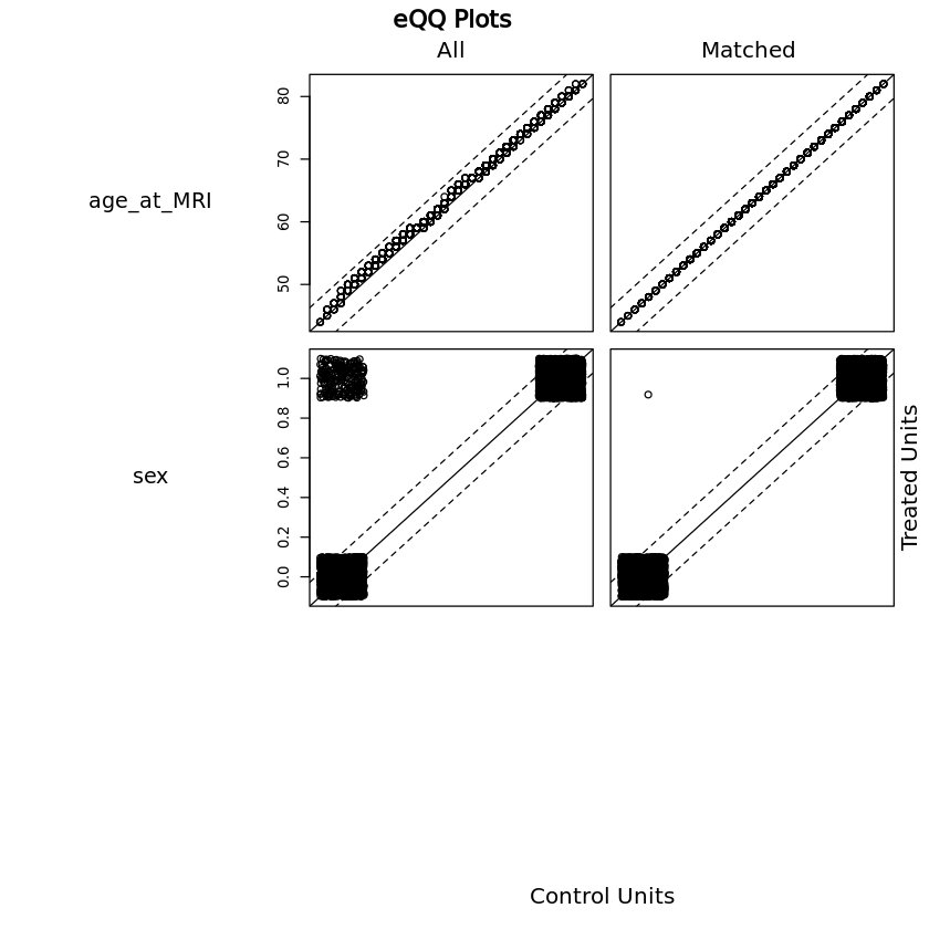
Dimensions of matched data (equal numbers in both groups once matched, number represents total of healthy + disease):

7338
136

Now compare distributions of matched data:

Warning message:
“`funs()` was deprecated in dplyr 0.8.0.
Please use a list of either functions or lambdas: 

  # Simple named list: 
  list(mean = mean, median = median)

  # Auto named with `tibble::lst()`: 
  tibble::lst(mean, median)

  # Using lambdas
  list(~ mean(., trim = .2), ~ median(., na.rm = TRUE))
This warning is displayed once every 8 hours.
Call `lifecycle::last_lifecycle_warnings()` to see where this warning was generated.”

A tibble: 2 × 2
rf_diabetes	sex
<dbl>	<dbl>
0	0.5500136
1	0.5500136

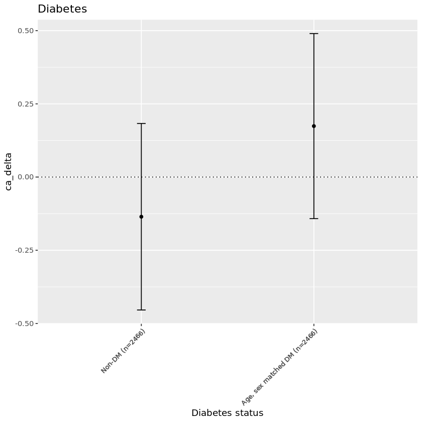
(ii) analysis#

Summary:#

A tibble: 2 × 3
rf_diabetes	meanca_delta	n
<dbl>	<chr>	<int>
0	-0.135	3669
1	0.174	3669

Plot:#

Regression (adjusted for age, age^2, sex):#

Call:
lm(formula = ca_delta ~ rf_diabetes + poly(age_at_MRI, 2) + sex, 
    data = dta_m)

Residuals:
    Min      1Q  Median      3Q     Max 
-33.248  -6.850  -0.218   6.791  34.131 

Coefficients:
                     Estimate Std. Error t value Pr(>|t|)  
(Intercept)            0.1550     0.2055   0.754   0.4507  
rf_diabetes            0.3096     0.2289   1.353   0.1762  
poly(age_at_MRI, 2)1  -4.3951     9.8172  -0.448   0.6544  
poly(age_at_MRI, 2)2  11.8102     9.8023   1.205   0.2283  
sex                   -0.5282     0.2304  -2.293   0.0219 *
---
Signif. codes:  0 ‘***’ 0.001 ‘**’ 0.01 ‘*’ 0.05 ‘.’ 0.1 ‘ ’ 1

Residual standard error: 9.802 on 7333 degrees of freedom
Multiple R-squared:  0.001205,	Adjusted R-squared:  0.0006602 
F-statistic: 2.212 on 4 and 7333 DF,  p-value: 0.06514

A matrix: 5 × 2 of type dbl
	2.5 %	97.5 %
(Intercept)	-0.2478601	0.55792884
rf_diabetes	-0.1390727	0.75818057
poly(age_at_MRI, 2)1	-23.6397501	14.84949413
poly(age_at_MRI, 2)2	-7.4051133	31.02549636
sex	-0.9797560	-0.07659024

Call:
lm(formula = ca_delta ~ poly(age_at_MRI, 2) + sex * rf_diabetes, 
    data = dta_m)

Residuals:
    Min      1Q  Median      3Q     Max 
-33.316  -6.844  -0.200   6.812  34.063 

Coefficients:
                     Estimate Std. Error t value Pr(>|t|)
(Intercept)           0.08751    0.24135   0.363    0.717
poly(age_at_MRI, 2)1 -4.39513    9.81772  -0.448    0.654
poly(age_at_MRI, 2)2 11.81019    9.80277   1.205    0.228
sex                  -0.40541    0.32555  -1.245    0.213
rf_diabetes           0.44460    0.34118   1.303    0.193
sex:rf_diabetes      -0.24553    0.46004  -0.534    0.594

Residual standard error: 9.803 on 7332 degrees of freedom
Multiple R-squared:  0.001244,	Adjusted R-squared:  0.0005628 
F-statistic: 1.826 on 5 and 7332 DF,  p-value: 0.1041

A matrix: 6 × 2 of type dbl
	2.5 %	97.5 %
(Intercept)	-0.3856115	0.5606381
poly(age_at_MRI, 2)1	-23.6406891	14.8504331
poly(age_at_MRI, 2)2	-7.4060508	31.0264339
sex	-1.0435851	0.2327641
rf_diabetes	-0.2242198	1.1134120
sex:rf_diabetes	-1.1473452	0.6562948

Call:
lm(formula = ca_delta ~ poly(age_at_MRI, 2) + I(1 - sex) * rf_diabetes, 
    data = dta_m)

Residuals:
    Min      1Q  Median      3Q     Max 
-33.316  -6.844  -0.200   6.812  34.063 

Coefficients:
                       Estimate Std. Error t value Pr(>|t|)
(Intercept)             -0.3179     0.2183  -1.456    0.145
poly(age_at_MRI, 2)1    -4.3951     9.8177  -0.448    0.654
poly(age_at_MRI, 2)2    11.8102     9.8028   1.205    0.228
I(1 - sex)               0.4054     0.3256   1.245    0.213
rf_diabetes              0.1991     0.3086   0.645    0.519
I(1 - sex):rf_diabetes   0.2455     0.4600   0.534    0.594

Residual standard error: 9.803 on 7332 degrees of freedom
Multiple R-squared:  0.001244,	Adjusted R-squared:  0.0005628 
F-statistic: 1.826 on 5 and 7332 DF,  p-value: 0.1041

A matrix: 6 × 2 of type dbl
	2.5 %	97.5 %
(Intercept)	-0.7458100	0.1100155
poly(age_at_MRI, 2)1	-23.6406891	14.8504331
poly(age_at_MRI, 2)2	-7.4060508	31.0264339
I(1 - sex)	-0.2327641	1.0435851
rf_diabetes	-0.4058792	0.8040210
I(1 - sex):rf_diabetes	-0.6562948	1.1473452

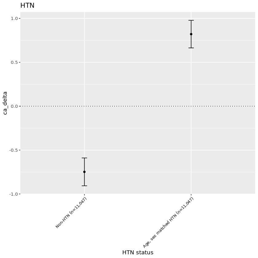
Disease 2: Hypertension#

(i) propensity match samples#

Healthy sample is matched to disease sample by age and sex.

First, examine if there are any differences in covariates.

	Welch Two Sample t-test

data:  age_at_MRI by rf_htn
t = -27.257, df = 32186, p-value < 2.2e-16
alternative hypothesis: true difference in means between group 0 and group 1 is not equal to 0
95 percent confidence interval:
 -2.376973 -2.058054
sample estimates:
mean in group 0 mean in group 1 
       63.03944        65.25696 

	Welch Two Sample t-test

data:  sex by rf_htn
t = -13.35, df = 31921, p-value < 2.2e-16
alternative hypothesis: true difference in means between group 0 and group 1 is not equal to 0
95 percent confidence interval:
 -0.08336211 -0.06201811
sample estimates:
mean in group 0 mean in group 1 
      0.4625790       0.5352692 

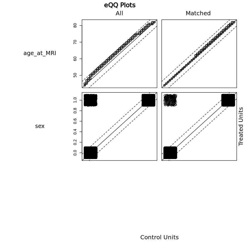
Dimensions of matched data (equal numbers in both groups once matched, number represents total of healthy + htn)

29686
137

Now compare distributions of matched data

A tibble: 2 × 2
rf_htn	sex
<dbl>	<dbl>
0	0.5226706
1	0.5352692

(ii) analysis#

Summary:#

A tibble: 2 × 3
rf_htn	mean_ca_delta	n
<dbl>	<chr>	<int>
0	-0.748	14843
1	0.821	14843

Plot:#

Regression (adjusted for age, age^2, sex):#

Call:
lm(formula = ca_delta ~ rf_htn + age_at_MRI + poly(age_at_MRI, 
    2) + sex, data = dta_m_htn)

Residuals:
    Min      1Q  Median      3Q     Max 
-36.609  -6.815  -0.133   6.809  34.599 

Coefficients: (1 not defined because of singularities)
                      Estimate Std. Error t value Pr(>|t|)    
(Intercept)           0.074600   0.517591   0.144    0.885    
rf_htn                1.571240   0.113906  13.794  < 2e-16 ***
age_at_MRI           -0.007320   0.007857  -0.932    0.352    
poly(age_at_MRI, 2)1        NA         NA      NA       NA    
poly(age_at_MRI, 2)2 22.142638   9.809253   2.257    0.024 *  
sex                  -0.657250   0.114046  -5.763 8.34e-09 ***
---
Signif. codes:  0 ‘***’ 0.001 ‘**’ 0.01 ‘*’ 0.05 ‘.’ 0.1 ‘ ’ 1

Residual standard error: 9.802 on 29681 degrees of freedom
Multiple R-squared:  0.007692,	Adjusted R-squared:  0.007559 
F-statistic: 57.52 on 4 and 29681 DF,  p-value: < 2.2e-16

A matrix: 6 × 2 of type dbl
	2.5 %	97.5 %
(Intercept)	-0.93990066	1.089100481
rf_htn	1.34797958	1.794500451
age_at_MRI	-0.02272063	0.008080425
poly(age_at_MRI, 2)1	NA	NA
poly(age_at_MRI, 2)2	2.91607216	41.369203679
sex	-0.88078623	-0.433714697

Call:
lm(formula = ca_delta ~ poly(age_at_MRI, 2) + sex * rf_htn, data = dta_m_htn)

Residuals:
    Min      1Q  Median      3Q     Max 
-36.587  -6.825  -0.133   6.808  34.579 

Coefficients:
                     Estimate Std. Error t value Pr(>|t|)    
(Intercept)          -0.42371    0.11647  -3.638 0.000275 ***
poly(age_at_MRI, 2)1 -9.03378    9.81466  -0.920 0.357352    
poly(age_at_MRI, 2)2 22.21658    9.81141   2.264 0.023559 *  
sex                  -0.61495    0.16113  -3.817 0.000136 ***
rf_htn                1.61602    0.16581   9.746  < 2e-16 ***
sex:rf_htn           -0.08477    0.22811  -0.372 0.710169    
---
Signif. codes:  0 ‘***’ 0.001 ‘**’ 0.01 ‘*’ 0.05 ‘.’ 0.1 ‘ ’ 1

Residual standard error: 9.802 on 29680 degrees of freedom
Multiple R-squared:  0.007697,	Adjusted R-squared:  0.00753 
F-statistic: 46.04 on 5 and 29680 DF,  p-value: < 2.2e-16

A matrix: 6 × 2 of type dbl
	2.5 %	97.5 %
(Intercept)	-0.6519931	-0.1954327
poly(age_at_MRI, 2)1	-28.2709396	10.2033823
poly(age_at_MRI, 2)2	2.9857783	41.4473769
sex	-0.9307677	-0.2991345
rf_htn	1.2910183	1.9410220
sex:rf_htn	-0.5318870	0.3623382

Call:
lm(formula = ca_delta ~ poly(age_at_MRI, 2) + sex * rf_htn, data = dta_m_htn)

Residuals:
    Min      1Q  Median      3Q     Max 
-36.587  -6.825  -0.133   6.808  34.579 

Coefficients:
                     Estimate Std. Error t value Pr(>|t|)    
(Intercept)          -0.42371    0.11647  -3.638 0.000275 ***
poly(age_at_MRI, 2)1 -9.03378    9.81466  -0.920 0.357352    
poly(age_at_MRI, 2)2 22.21658    9.81141   2.264 0.023559 *  
sex                  -0.61495    0.16113  -3.817 0.000136 ***
rf_htn                1.61602    0.16581   9.746  < 2e-16 ***
sex:rf_htn           -0.08477    0.22811  -0.372 0.710169    
---
Signif. codes:  0 ‘***’ 0.001 ‘**’ 0.01 ‘*’ 0.05 ‘.’ 0.1 ‘ ’ 1

Residual standard error: 9.802 on 29680 degrees of freedom
Multiple R-squared:  0.007697,	Adjusted R-squared:  0.00753 
F-statistic: 46.04 on 5 and 29680 DF,  p-value: < 2.2e-16

A matrix: 6 × 2 of type dbl
	2.5 %	97.5 %
(Intercept)	-0.6519931	-0.1954327
poly(age_at_MRI, 2)1	-28.2709396	10.2033823
poly(age_at_MRI, 2)2	2.9857783	41.4473769
sex	-0.9307677	-0.2991345
rf_htn	1.2910183	1.9410220
sex:rf_htn	-0.5318870	0.3623382

Forest plot: Categorical variables#

The CCIG Grimoire

Association analysis between risk factors and cardiovascular age-delta

Contents

Association analysis between risk factors and cardiovascular age-delta#

Introduction#

Disease 1: Diabetes#

(i) propensity match samples#

(ii) analysis#

Summary:#

Plot:#

Regression (adjusted for age, age^2, sex):#

Disease 2: Hypertension#

(i) propensity match samples#

(ii) analysis#

Summary:#

Plot:#

Regression (adjusted for age, age^2, sex):#

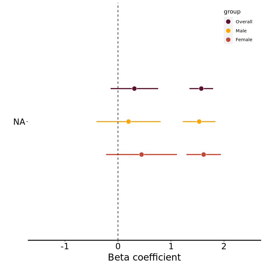
Forest plot: Categorical variables#